Original source: Complete guide to understanding Node2Vec algorithm
Machine learning has become a vital tool in our everyday life. Almost a day doesn’t go by when you don’t use any of the wide range of applications that use machine learning in one way or another. If you have some experience with training machine learning models, you might be used to having the underlying training data stored in the form of a table. However, we live in an era where the world is more connected than ever before. Not only is the world connected, but the data we collect is more and more related. Storing the data in a table form has the downside of possibly neglecting the relationships that might be relevant and predictable in your application. Here is where the graph store comes in. By design, you need to consider possible connections between your data points when constructing a graph.
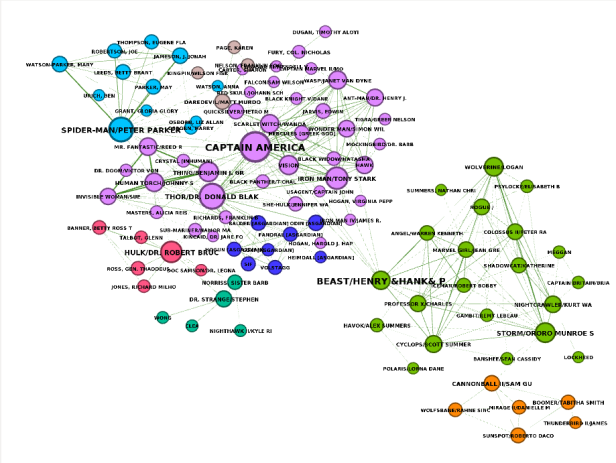
Visualization of a Marvel character network. Image by the author.
A graph consists of nodes and their relationships. This simple yet very effective way of storing the data allows you to model almost any real-world scenario. Networks are the core of the internet, transportation, social platforms, and so on. A graph can represent protein interactions, chemical bonds, road networks, social networks, and many others. Now, what does this have to do with machine learning? In recent years, a lot of research was made on extracting network structure and using it in machine learning applications. For example, the researchers from DeepMind, Google Brain, MIT, and University of Edinburgh argue in their research paper that graph networks can support two critical capabilities, which are a top priority for AI to achieve human-like abilities:
- Relational reasoning: Explaining relationships between different entities, such as image pixels, words, proteins or others
- Combinatorial Generalization: Constructing new inferences, predictions, and behaviors from known building blocks.
A typical input for a machine learning model is a vector that represents each data point. The process of translating relationships and network structure into a set of vectors is named node embedding. A node embedding algorithm aims to encode each node into an embedding space while preserving the network structure information. Encoding entity relationships allows you to capture the context of each data point rather than just focusing on its attributes. And we all know that context is king!
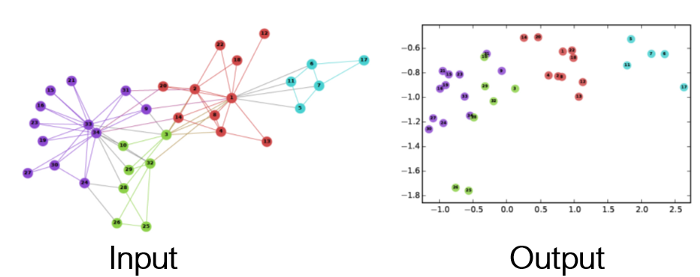
Graph Embedding — Representation Learning on Networks, snap.stanford.edu/proj/embeddings-www
You might have already dealt with graphs before in a more classical ML setup. Any image can be represented as a grid graph.
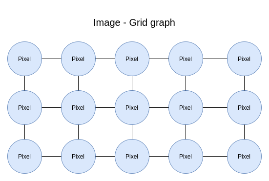
Any image can be represented as a grid graph. Image by the author.
In image processing and classification, convolutional neural networks are often used. But what exactly is a convolution? I like this quote from Dr. Prasad Samarakoon:
A convolution can be thought as “looking at a function’s surroundings to make better/accurate predictions of its outcome.
Essentially, a convolution examines the relationships between pixels to capture the deeper, contextual meaning of images. Similarly, you can represent any text as a graph.
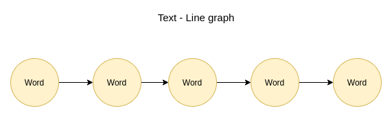
Any text can be represented as a line graph. Image by the author.
If you’ve ever dealt with word embedding, you know that you can capture word meaning and function by examining its surrounding. Node embedding algorithms try to generalize what word and image embedding do on any graph structure. Real-world networks don’t have a predefined structure and can be of various shapes and sizes. The output of a node embedding algorithm can then be used as an input to a downstream machine learning model. For example, node2vec is a node embedding algorithm. In this blog post, I will try to present how node2vec algorithm is implemented.
Word2vec Skip-gram model
The node2vec algorithm is heavily inspired by the word2vec skip-gram model. Therefore, to properly understand node2vec, you must first understand how the word2vec algorithm works. Word2Vec is a shallow, two-layer neural network that is trained to reconstruct linguistic contexts of words. The objective of the word2vec model is to produce word representation (vectors) given a text corpus. Word representations are positioned in the embedding space such that words that share common contexts in the text corpus are located close to one another in the embedding space. There are two main models used within the context of word2vec.
- Continuous Bag-of-Words (CBOW)
- Skip-gram model
Node2vec is inspired by the skip-gram model, so we will skip the CBOW implementation explanation. The Skip-gram model predicts the context for a given word. The context is defined as the adjacent words to the input term.
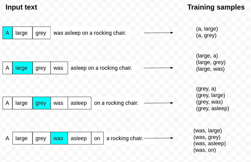
Context window. Image by the author.
The word highlighted in blue is the input term. In this example, the context window size is five. Window size is defined as the maximum distance between words in the context window with the input word in the center. In practice, it seems that the norm is to use the context words adjacent to half of the window size from the input word. As you can see by the first example in the image, we only use the following two words as the context, even though the context size is five.
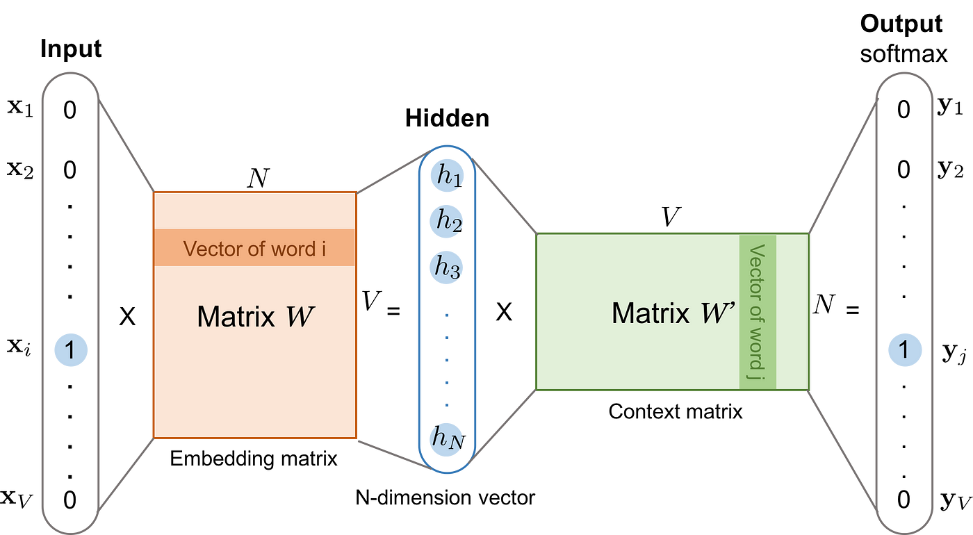
The skip-gram model. Image from https://lilianweng.github.io/lil-log/2017/10/15/learning-word-embedding.html. Posted with permission from the author.
In this image, the architecture of the skip-gram neural network is presented. When training this neural network, the input is a one-hot encoded vector representing the input word, and the output is also a one-hot encoded vector representing the context word. Remember from the previous image how we constructed input and context pairs of words. Word2vec uses a trick where we aren’t interested in the output vector of the neural network, but rather the goal is to learn the weights of the hidden layer. The weights of the hidden layer are actually the word embedding we are trying to learn. The number of neurons in the hidden layer will determine the embedding dimension or the size of the vector representing each word in the vocabulary.
Note that the neural network does not consider the offset of the context word, so it does not differentiate between directly adjacent context words to the input and those more distant in the context window or even if the context word precedes or follows the input term. Consequently, the window size parameter has a significant influence on the results of the word embedding. For example, a study Dependency-Based Word Embeddings by Levy & Goldberg finds that larger context window size tends to capture more topic/domain information. In contrast, smaller windows tend to capture more information about the word itself, e.g., what other words are functionally similar.
Negative sampling and subsampling
The authors of the word2vec skip-gram model have later published a Distributed representations of words and phrases and their compositionality that introduces two optimizations to the original model. The first optimization is the subsampling of frequent words. In any text corpus, the most frequent terms will most likely be the so-called stop words like “the”, “at”, “in”. While the skip-gram model benefits from co-occurrences of words like “Germany” and “Berlin”, the benefit of frequent co-occurrences of “Germany” and “the” is far smaller as nearly every word is accompanied with “the” term. The authors implemented a subsampling technique to address this issue. For each word in the training corpus, there is a chance that we will ignore specific instances of the word in the text. The probability of cutting the word from a sentence is related to the word’s frequency. The research paper shows that subsampling of frequent words during training results in a significant speedup and improves the representations of less frequent words.
The second optimization is the introduction of negative sampling. Training a neural network involves taking a training sample and adjusting all of the neuron weights to predict that training sample more precisely. In layman’s terms, each training sample will tweak all of the weights in the neural network. A Test Your Vocab study shows that most adult native speakers’ vocabulary ranges from 20,000–35,000 words and you can have millions or even billions of input-context training pairs. Updating several thousand weights for every input-context training pair is very expensive. Negative sampling solves this performance issue by having each training sample modify only a small subset of the weights rather than all of them. With negative sampling, a “negative” word is one for which we want the neural network to output a 0, meaning that it is not in the context of our input term. We will still update the weights for our “positive” context word. Experiments indicate that the number of negative samples in the range 5–20 is useful for small training datasets. For larger datasets, the number of negative examples can be as small as 2–5. So, for example, instead of updating all of the neuron weights for each training sample, we only update five negative and one positive weight. This will have a significant impact on the model training time. The paper shows that selecting negative samples using the unigram distribution raised to the 3/4rd power significantly outperformed other options. In a unigram distribution, more frequent words are more probable to be selected as negative samples.
I have found this excellent Considerations about learning Word2Vec study that delves into word2vec hyper-parameter optimization. You have already discovered what do context window size, embedding dimension, and negative samples mean, but the authors have also looked at the influence of the neural network learning rate on embedding results.
Node2vec
Node2vec algorithm uses skip-gram with negative sampling (SGNS). But how do we create a text corpus as input to the SGNS? Node2vec uses random walks to generate a corpus of “sentences” from a given network.
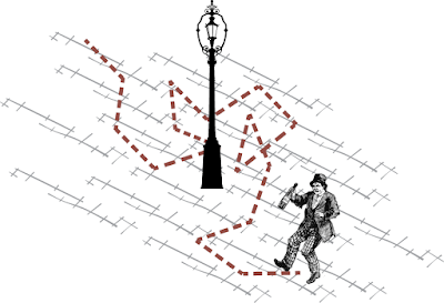
Image source: https://prakhartechviz.blogspot.com/2019/09/random-walk-term-weighting-for-text.html
A random walk can be interpreted as a drunk person traversing the graph. Of course, you can never be sure of an intoxicated person’s next step, but one thing is sure. A drunk person traversing the graph can only hop onto a neighboring node.
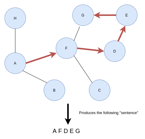
Construct sentences based on random walks. Image by the author.
Imagine if you start traversing the graph from node A. At random, you pick a neighboring node and hop on to it. Then you repeat the process until a predefined walk length. The walk length parameter defines how long the “sentences” will be. For every node in the graph, the node2vec algorithm generates a series of random walks with the particular node as the starting node. You can define how many random walks should start from a particular node with the walks per node parameter. To sum it up, the node2vec algorithm uses random walks to generate a number of sentences starting from each node in the graph. The walk length parameter controls the length of the sentence. Once the sentences are generated using random walks, the algorithm inputs them into the SGNS model and retrieve the hidden layer weights as node embeddings. That is the whole gist of the node2vec algorithm.
However, the node2vec algorithm implements second-order biased random walks. A step in the first-order random walk only depends on its current state.
First-order random walks
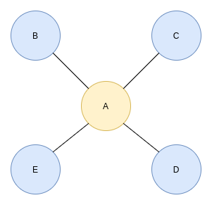
First-order random walk. Image by the author.
Imagine you have somehow wound up at node A. Because the first-order random walk only looks at its current state, the algorithm doesn’t know which node it was at the earlier step. Therefore, the probability of returning to a previous node or any other node is equal. There is no advanced math concept behind the calculation of probability. Node A has four neighbors, so the chance of traversing to any of them is 25% (1/4).
Suppose your graph is weighted, meaning that each relationship has a property that stores its weight. In that case, those weights will be included in the calculation of the traversal probability.
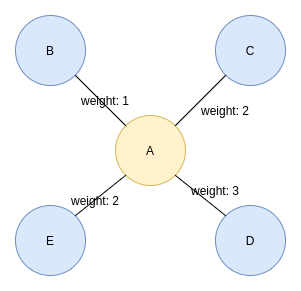
First-order random walk on a weighted graph. Image by the author.
In a weighted graph, the chance of traversing a particular connection is its weight divided by the sum of all neighboring weights. For example, the probability to traverse from node A to node E is 2 divided by 8 (25%) and the probability to traverse from node A to node D is 37.5%.
Second-order biased random walks
Second-order walks take into account both the current as well as the previous state. To put it simply, when the algorithm calculates the traversal probabilities, it also considers where it was at the previous step.
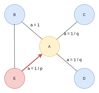
Second-order biased random walk. Image by the author.
The walk just traversed from node E to node A in the previous step and is now evaluating its next move. The likelihood of backtracking the walk and immediately revisiting a node in the walk is controlled by the return parameter p. Setting a high value to parameter p ensures lower chances of revisiting a node and avoids 2-hop redundancy in sampling. This strategy also encourages moderate graph exploration. On the other hand, if the value of the p parameter is low, the chances of backtracking in the walk are higher, keeping the random walk closer to the starting node.
The inOut parameter q allows the traversal calculation to differentiate between inward and outward nodes. Setting a high value to parameter q (q > 1) biases the random walk to move towards nodes close to the node in the previous step. Going to the previous image, if you set a high value for parameter q, the random walk from node A is biased towards nodes closer to node E. Such walks obtain a local view of the underlying graph with respect to the starting node in the walk and approximate breadth-first search. In contrast, if the value of q is low (q < 1), the walk is more inclined to visit nodes further away from node E. This strategy encourages outward exploration and approximates depth-first search.
Homophily vs structural equivalence
Various configurations of the return and inOut parameters in the second-order biased random walks produce different similarities between nodes. Specifically, you can tune the node2vec to follow homophily similarity**.** In this context, homophily is defined as nodes that belong to the same network community (i.e., are closer to one another in the network). Homophily can be achieved by setting a smaller value of q. A smaller value of q approximates depth-first search.
On the other hand, you can encourage more structural equivalence similarity by setting a higher value of q. Structural equivalence refers to the extent to which two nodes are connected to the same nodes, i.e., they share the same neighborhood while not requiring the two nodes to be directly connected. What is not intuitive at first glance is that structural equivalent nodes will also be regularly equivalent. Regular equivalence is defined as nodes that have similar connection patterns to other nodes. An example of that would be bridge nodes in the network. For more information about structural and regular equivalence, read the Community detection in graphs paper.
node2vec: Scalable Feature Learning for Networks. A. Grover, J. Leskovec. ACM SIGKDD International Conference on Knowledge Discovery and Data Mining (KDD), 2016.
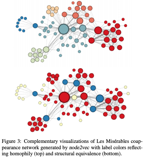
The best explanation of this figure are the authors’ own words:
Figure 3(top) shows the example when we set p = 1, q = 0.5. Notice how regions of the network (i.e., network communities) are colored using the same color. In this setting node2vec discovers clusters/communities of characters that frequently interact with each other in the major sub-plots of the novel. Since the edges between characters are based on coappearances, we can conclude this characterization closely relates with homophily. In order to discover which nodes have the same structural roles we use the same network but set p = 1, q = 2, use node2vec to get node features and then cluster the nodes based on the obtained features. Here node2vec obtains a complementary assignment of node to clusters such that the colors correspond to structural equivalence as illustrated in Figure 3(bottom). For instance, node2vec embeds blue-colored nodes close together. These nodes represent characters that act as bridges between different sub-plots of the novel. Similarly, the yellow nodes mostly represent characters that are at the periphery and have limited interactions
Node2vec details
Before I let you go, I want to share some of the high-level node2vec implementation consequences. First of all, the node2vec algorithm does not differentiate between node or relationship types. If your graph has many node or relationship types, the node2vec algorithm will not consider that. Secondly, node properties or features cannot be added to the algorithm input. The resulting node embeddings are only affected by the network topology and not node properties or attributes.
Last, but not least, the node2vec algorithm is a transductive node embedding algorithm, meaning that, it needs the whole graph to be available to learn the node embeddings. You cannot run the node2vec algorithm separately on your test and training data. Similarly, when a new node is added to your graph, you need to rerun the node2vec algorithm on the whole graph if you want to generate embedding for the new node.
Summary
Node2vec algorithm can be summarized as a two-part process. First, it uses second-order biased random walks to generate sequences of nodes or “sentences”. By fine-tuning random walk hyper-parameters, you can influence the random walk length and whether you want to encapsulate more of a homophily or structural equivalence similarity. Second, once the sequences of nodes are generated, they are used as an input to a skip-gram with negative sampling model. The skip-gram model first generates pairs of input and context nodes given the context window size and then feeds them into a shallow two-layer neural network. Once the neural network is trained, you can retrieve the hidden layer weights as your node embeddings. The number of neurons in the hidden layer will determine the size of the embedding.
References
- Tomas Mikolov, Kai Chen, Greg Corrado, Jeffrey Dean: Efficient Estimation of Word Representations in Vector Space, 2013, arXiv:1301.3781
- P. Battaglia et al., Relational inductive biases, deep learning, and graph networks (2018), arXiv:1806.01261.
- node2vec: Scalable Feature Learning for Networks. A. Grover, J. Leskovec. ACM SIGKDD International Conference on Knowledge Discovery and Data Mining (KDD), 2016.
- McCormick, C. (2016, April 19). Word2Vec Tutorial — The Skip-Gram Model. Retrieved from http://www.mccormickml.com
- Fortunato, S… “Community detection in graphs.” ArXiv abs/0906.0612 (2009): n. pag.
- Di Gennaro, G., Buonanno, A. & Palmieri, F.A.N. Considerations about learning Word2Vec. J Supercomput (2021). https://doi.org/10.1007/s11227-021-03743-2
- Levy, Y. (2014). Dependency-Based Word Embeddings. In Proceedings of the 52nd Annual Meeting of the Association for Computational Linguistics (Volume 2: Short Papers) (pp. 302–308). Association for Computational Linguistics.