In recommender systems, feature crossing and feature selection are eternal topics. From the hand-crafted feature interactions of the logistic regression era, to the exhaustive feature interactions of poly2, to the latent-vector feature interactions of FM, and then to the automatic feature interactions of GBDT+LR — this is the history of feature engineering before deep learning methods came along.

After ResNet solved the vanishing gradient problem caused by excessive network depth in 2014, deep neural networks were widely adopted in industry. In 2016, Microsoft released the Deep Crossing model for binary classification tasks such as CTR prediction. A link to the original paper is below: Deep Crossing: Web-Scale Modeling without Manually Crafted Combinatorial Features

Paper Walkthrough

The name alone tells you what it sets out to solve: the problem of manually constructing combinatorial features. It achieves deep feature crossing by building a network. Deep Crossing supports text, categorical, ID, and numerical features.

The network architecture of Deep Crossing is as follows:

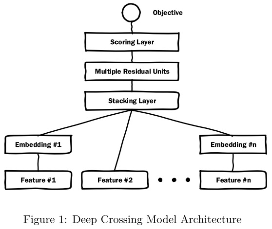
There are four core parts: the Embedding layer, which embeds the features; the Stacking layer, which simply concatenates the embeddings together; then multiple Residual blocks that extract features. Finally, a Scoring layer produces the score — that is, the resulting logit value. Sorting by this logit value gives the ranking of the ads to be served.

In the original paper, the features Microsoft used are shown below:

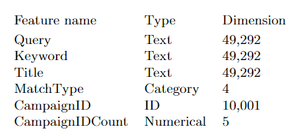
Some of the key concepts are also explained:

Feature	Meaning
Query	The search term the user types into the search box
Keyword	A keyword the advertiser attaches to an ad to describe its product
Title	The ad title
Landing Page	The page the user lands on after clicking the ad
Match Type	The ad-to-query matching type chosen by the advertiser (exact, broad, semantic, etc.)
Click Through Rate	The ad’s historical click-through rate
Click Prediction	The CTR estimate from another CTR model
Campaign	The ad delivery plan created by the advertiser, including budget, targeting conditions, and so on
Impression	An example of an ad impression, recording information about the ad in an actual impression context
Click	An example of an ad click, recording information about the ad in an actual click context

Every individual feature is converted into a vector. For text features like Query, for example, the result is a 49,292-dimensional vector. Low-cardinality categorical inputs such as match type are handled with one-hot encoding. For high-cardinality features such as Campaign ID, which represents different ad campaigns and typically has millions of distinct IDs, the original author’s approach is to pick the top 10,000 by historical click-through rate, number them from 0 to 9,999, and assign a single shared ID of 10,001 to everything else. A derived feature is built alongside it: the historical CTRs of all IDs are combined into a 10,001-dimensional dense matrix, where each element is the historical CTR of the corresponding ID and the last element is the average CTR of the remaining IDs. Reducing dimensionality while introducing derived features like this is an effective way to curb the explosion in parameter count that high-cardinality features cause.

This is also where the 10,001 dimensions shown for Campaign ID in the original figure come from.

The paper doesn’t explain feature embedding very clearly, and after going through many explanations online I still don’t fully understand this part. The original text includes a few tricks tailored to its own scenario, but the overall idea is to embed a high-dimensional sparse matrix into a low-dimensional dense one.

After the embedding layer, the Stacking layer concatenates everything and passes it straight to the residual layers.

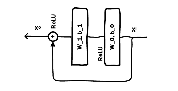
For the residual blocks from ResNet, the original convolution kernels are replaced with ordinary MLP layers. After passing through multiple residual layers, the model outputs a score used to judge whether a user will click the corresponding ad.

Implementation

Let’s implement this in PyTorch. Assuming feature engineering and preprocessing are already done, we need to implement the dataset class, the model, and the training/prediction code:

class CustomDataset(Dataset):
    def __init__(self, X, y=None):
        self.X = X  # Dataframe
        self.y = y
        
    def __len__(self):
        return len(self.X)
    
    def __getitem__(self, index):
        X_item = torch.tensor(self.X.iloc[index].values, dtype=torch.float32)
        if self.y is not None:
            y_item = torch.tensor(self.y.iloc[index], dtype=torch.float32)
            return X_item, y_item
        return X_item
        
        
train_dataset = CustomDataset(X_train, y_train)
test_dataset = CustomDataset(X_test, y_test)

train_loader = DataLoader(train_dataset, batch_size=32, shuffle=True)
test_loader = DataLoader(test_dataset, batch_size=32, shuffle=False)

Defining the model:

class DeepCrossing(nn.Module):
    def __init__(self, input_dims, embedding_dim, residual_dims, output_dim=1):
        super(DeepCrossing, self).__init__()
        
        # 对每维特征进行嵌入
        self.embeddings = nn.ModuleList([
            nn.Linear(input_dim, embedding_dim) if input_dim > embedding_dim else nn.Identity()
            for input_dim in input_dims
        ])
        
        # Stacking layer
        self.stack_dim = sum(embedding_dim if input_dim > embedding_dim else input_dim for input_dim in input_dims)
        
        # 残差块
        self.residual_units = nn.Sequential(
            *[ResidualUnit(self.stack_dim, dim) for dim in residual_dims]
        )
        
        # 评分层
        self.scoring_layer = nn.Linear(self.stack_dim, output_dim)
        
    def forward(self, inputs):
        embedded = [embedding(input) for embedding, input in zip(self.embeddings, inputs)]
        # 直接concat特征
        stacked = torch.cat(embedded, dim=1)
        
        out = self.residual_units(stacked)
        out = torch.sigmoid(self.scoring_layer(out))
        return out

class ResidualUnit(nn.Module):
    def __init__(self, input_dim, hidden_dim):
        super(ResidualUnit, self).__init__()
        self.fc1 = nn.Linear(input_dim, hidden_dim)
        self.fc2 = nn.Linear(hidden_dim, input_dim)
        
    def forward(self, x):
        residual = x
        out = F.relu(self.fc1(x))
        out = self.fc2(out)
        out += residual
        return F.relu(out)

Next, the training portion:

# 假设输入维度是10
input_dims = 10

embedding_dim = 8
residual_dims = [64, 128, 64, 32]

model = DeepCrossing(input_dims, embedding_dim, residual_dims)

# 4. 训练模型
criterion = nn.BCELoss()
optimizer = optim.Adam(model.parameters(), lr=0.001)

def train(model, train_loader, criterion, optimizer, num_epochs=10):
    model.train()
    for epoch in range(num_epochs):
        running_loss = 0.0
        for inputs, labels in train_loader:
            inputs = [inputs[:, i].unsqueeze(1) for i in range(inputs.shape[1])]
            
            optimizer.zero_grad()
            outputs = model(inputs).squeeze()
            loss = criterion(outputs, labels)
            loss.backward()
            optimizer.step()
            running_loss += loss.item() * inputs[0].size(0)
        
        epoch_loss = running_loss / len(train_loader.dataset)
        print(f'Epoch {epoch+1}/{num_epochs}, Loss: {epoch_loss:.4f}')

train(model, train_loader, criterion, optimizer)

Model evaluation:

def evaluate(model, test_loader):
    model.eval()
    predictions = []
    with torch.no_grad():
        for inputs, labels in test_loader:
            inputs = [inputs[:, i].unsqueeze(1) for i in range(inputs.shape[1])]
            outputs = model(inputs).squeeze()
            predictions.extend(outputs.tolist())
    return predictions

predictions = evaluate(model, test_loader)
predictions = np.array(predictions) > 0.5  # 将输出转换为二分类预测
print("Predictions: ", predictions)

August 18, 2024, in Suzhou