3D Reconstruction: Starting with Stereo Matching

I have written less and less in 2026. Partly, my motivation for studying recommender systems has waned—especially after generative retrieval raised the bar for data volume and multi-GPU clusters, making industrial-scale models difficult to reproduce locally. I have also spent a great deal of time researching stocks and have been less diligent about technical exploration. A fair self-criticism.

For a while, I did not want to look at recommender systems, so I started exploring subjects that interested me. 3D reconstruction is one of them. Because I know almost nothing about computer graphics, I decided to learn the field from the beginning. Much of this post comes from ChatGPT, online articles, and open-source projects, so some of my early interpretations may be inaccurate.

3D Reconstruction, U-Net, GANs, and Diffusion

When I first thought about reconstruction, models such as U-Net and GAN came to mind: add and remove noise from a 2D image, reduce the loss, and obtain a model. My initial assumption was that 3D reconstruction simply adds spatial dimensions to the data. The answer I got was that although these paradigms are used in the field, it is not that simple. Geometry, viewpoints, coordinate systems, consistency, and other physical-space constraints all matter.

One important issue is the explosion in data size. One extra dimension can mean an exponential increase; if each pixel also stores physical details and gradients, memory usage can far exceed that of 2D reconstruction. 3D reconstruction also requires consistency across viewpoints: the object must be recovered from all 360 degrees. These are fundamental challenges of the field.

Stereo Matching

Early 3D reconstruction applications mainly relied on stereo vision. By photographing the same object with a pair of cameras that mimic the positions of the left and right eyes, we find corresponding points in the two images, calculate their disparity, obtain a depth map—the distance from the object to the camera—and finally generate a point cloud or mesh. This gives a 2D image depth information.

Disparity is the positional difference of the same point in two images. It lets us infer distance, or depth. Calculate depth for every pixel and we obtain a collection of 3D points: a point cloud.

To calculate disparity, the same point must first be matched between the left and right images. This is the core of stereo matching. In broad terms, it uses a sliding-window-like procedure: take a small patch, find the most similar patch on the other side, score the match with a cost function—for example, a smaller grayscale difference means greater similarity—and choose the disparity with the lowest cost.

A stereo camera has two lenses, one on the left and one on the right. Their distance is the baseline, B. The camera focal length, f, is also known—for example, 800 pixels.

Once the two images are obtained, they need epipolar rectification. A point in the left image must correspond to some extended line in the right image; that line is the epipolar line. Rectification makes matching easier: after we know a point in the left image, we need only search along its epipolar line in the right image. The task then becomes finding the most similar position on that line for every left-image pixel.

With focal length, baseline, and disparity, a point’s depth can be recovered as focal length times baseline divided by disparity.

I made a small demo for stereo depth matching. Given rectified stereo images, a baseline, focal length, and related parameters, it returns a depth map and point cloud from the original image pair.

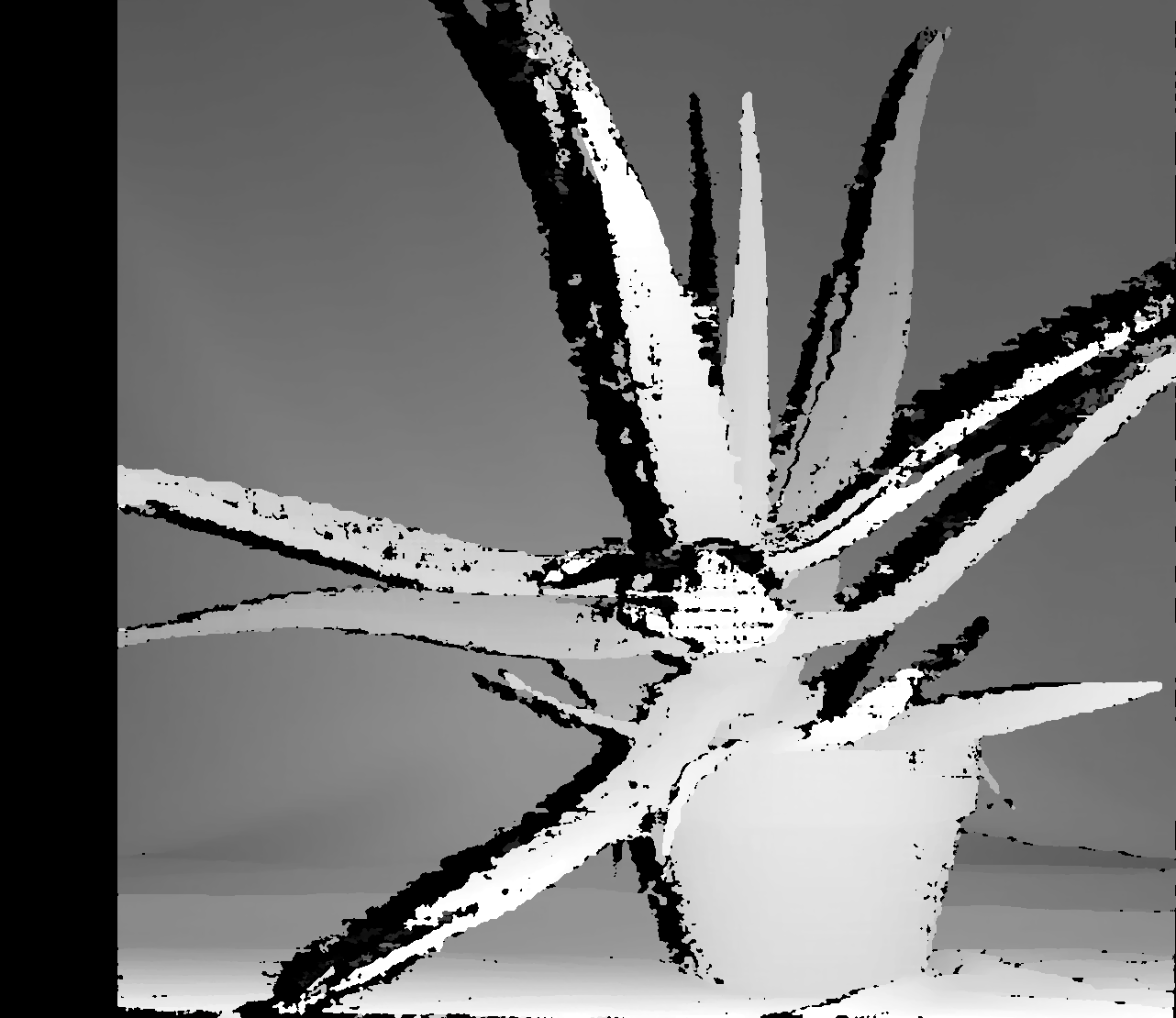
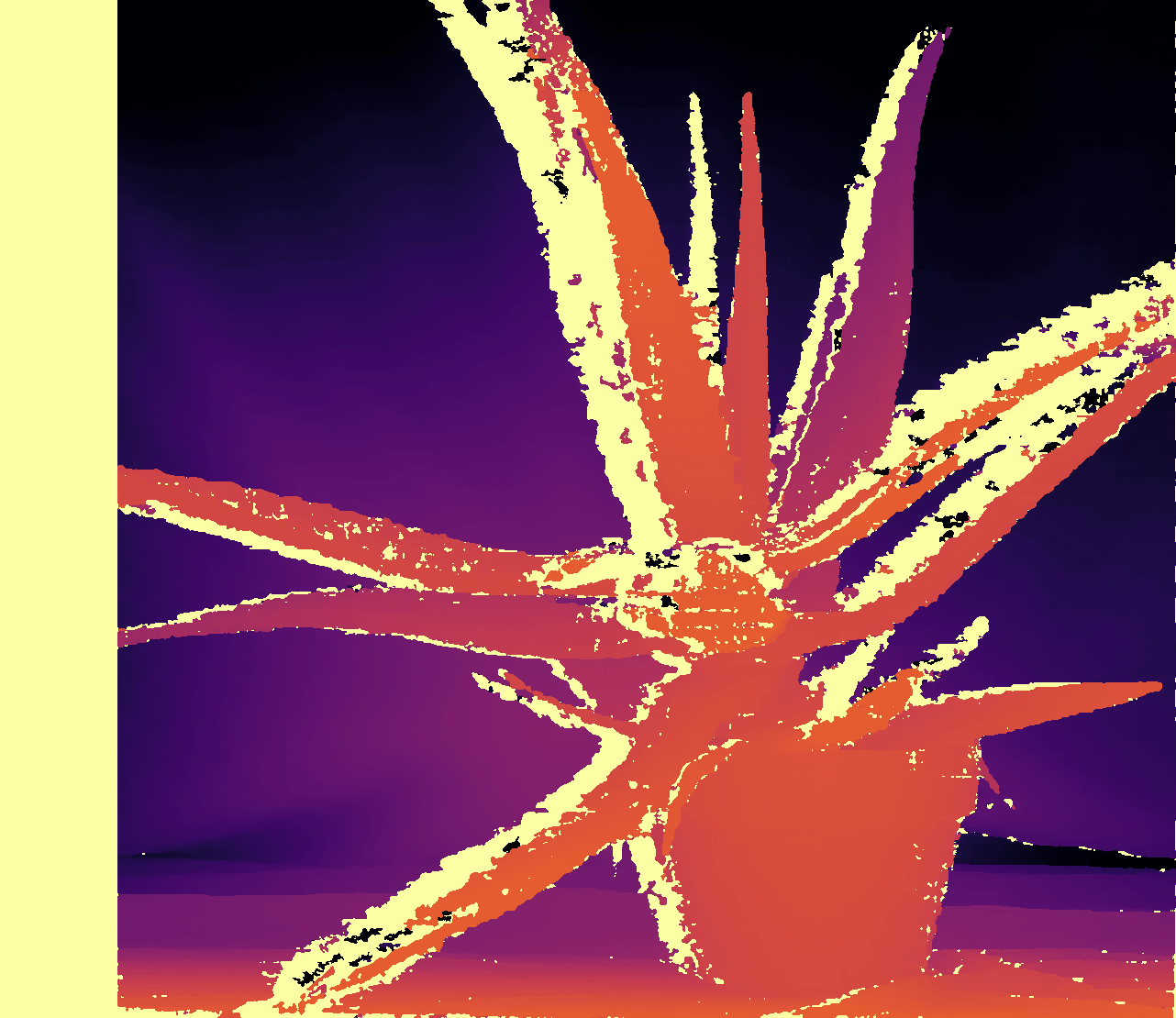
Stereo matching was popular in the early 2000s, but its performance depends strongly on matching accuracy and that creates many limits in practice.

Multi-View Reconstruction (MVS: Multi-View Stereo)

Stereo vision has only two images. Later work extended it to reconstruct a point cloud from many images: Multi-View Stereo (MVS).

The idea is the same. The same point appears at different locations in images taken by different cameras; the positional difference lets us infer depth.

In practice there are two parts. First estimate the pose of each camera, then perform matching using those poses. Once we know where many photos were taken, visual consistency among them can recover a dense 3D structure of the scene surface.

This involves SfM (Structure from Motion), which extracts camera intrinsics—focal length, principal point, distortion parameters, and image size—camera extrinsics—position and orientation—and a sparse point cloud from photographs taken at different angles. It then fuses the depth map from every image into a dense point cloud, depth map, or mesh.

A mesh is a grid of polygons used to form a 3D graphic. A model consists of multiple meshes; each mesh contains multiple polygons, usually triangles.

A related concept is the Gaussian. A 3D Gaussian resembles a semi-transparent ellipsoid. Layers of them approximate a scene as the human eye sees it. Compared with meshes, they favor visual realism over geometric precision.

The 3D world is represented by a set of 3D points—usually hundreds of thousands to millions. Every point is a 3D Gaussian with its own parameters, fitted so that rendering the scene closely matches known dataset images. --bimant

The MVS intuition is that a point viewed from different positions should have similar color and texture. Assume a pixel has depth d and corresponds to a 3D point P. When P is projected into the other photographs, its color and texture should remain similar. We take the depth whose projected appearances agree across the greatest number of images as the final depth.

The depth-estimation process is roughly:

• Try several candidate depths for every pixel.
• Project every candidate into the other images.
• Compare local texture consistency.
• Choose the depth with the strongest agreement.

Depth-Map Fusion

A depth map alone is not enough. A complete 3D model needs fusion: back-project every depth-map pixel into a 3D point with the camera parameters, merge duplicate points, remove inconsistent points, and obtain a dense point cloud.

After looking through projects on GitHub, I found that this is still an active field rather than an outdated one. There is continued work on matching acceleration, surface reconstruction, and many other improvements.

Structure from Motion (SfM)

SfM infers the relative poses of the cameras and the real-world 3D coordinates of object points from the pixel coordinates of the same object across a set of images. The result is a sparse 3D representation of the scene: a sparse point cloud.

Its input is multiple photographs; its output is each photograph’s camera pose, a sparse point cloud, and camera intrinsics. Compared with a dense point cloud, a sparse one is more like the key skeletal points used in human-pose estimation.

The first step is to find keypoints: visually distinctive points with unique textures, such as corners or holes. Feature matching then finds their counterparts in another image. Various methods filter bad matches along the way, for example by rejecting apparently similar points that do not lie on the relevant epipolar line.

SfM keypoint matching resembles stereo depth matching, but its goal differs. Stereo matching estimates depth for every pixel or patch; SfM only matches salient keypoints in order to recover camera rotation and translation. Those parameters are enough to locate the camera.

Once the camera positions and the pixel positions of feature points are known, we can infer 3D points. This uses triangulation: pixels in two photographs define rays from two cameras, and the real 3D point lies where the rays intersect.

This maps 3D points from two images. Repeating the same process over more photographs produces more sparse feature points.

Finally, a global optimization is needed to control the errors accumulated at every stage. It is called bundle adjustment. It reprojects the reconstructed 3D points back onto the photographs and compares them with the originals, optimizing until the difference is minimized.

To close, here is a useful visual summary:

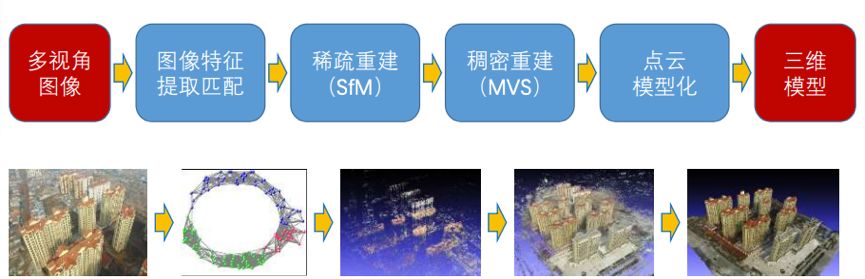
That is as far as I have gotten. I thought it would be straightforward, but the more I read, the more formulas and principles appeared. It is much deeper than I expected, and I will keep working through it gradually.

Suzhou, May 28, 2026